时间复杂度¶

统计算法运行时间¶

运行时间能够直观且准确地体现出算法的效率水平。如果我们想要 准确预估一段代码的运行时间 ，该如何做呢？

首先需要 确定运行平台 ，包括硬件配置、编程语言、系统环境等，这些都会影响到代码的运行效率。
评估 各种计算操作的所需运行时间 ，例如加法操作 + 需要 1 ns ，乘法操作 * 需要 10 ns ，打印操作需要 5 ns 等。
根据代码 统计所有计算操作的数量 ，并将所有操作的执行时间求和，即可得到运行时间。

例如以下代码，输入数据大小为 $n$ ，根据以上方法，可以得到算法运行时间为 $6n + 12$ ns 。

\[ 1 + 1 + 10 + (1 + 5) \times n = 6n + 12 \]

JavaC++PythonGoJavaScriptTypeScriptCC#

// 在某运行平台下
void algorithm(int n) {
    int a = 2;  // 1 ns
    a = a + 1;  // 1 ns
    a = a * 2;  // 10 ns
    // 循环 n 次
    for (int i = 0; i < n; i++) {  // 1 ns ，每轮都要执行 i++
        System.out.println(0);     // 5 ns
    }
}

// 在某运行平台下
void algorithm(int n) {
    int a = 2;  // 1 ns
    a = a + 1;  // 1 ns
    a = a * 2;  // 10 ns
    // 循环 n 次
    for (int i = 0; i < n; i++) {  // 1 ns ，每轮都要执行 i++
        cout << 0 << endl;         // 5 ns
    }
}

# 在某运行平台下
def algorithm(n):
    a = 2      # 1 ns
    a = a + 1  # 1 ns
    a = a * 2  # 10 ns
    # 循环 n 次
    for _ in range(n):  # 1 ns
        print(0)        # 5 ns

// 在某运行平台下
func algorithm(n int) {
    a := 2      // 1 ns
    a = a + 1   // 1 ns
    a = a * 2   // 10 ns
    // 循环 n 次
    for i := 0; i < n; i++ {    // 1 ns
        fmt.Println(a)          // 5 ns
    }
}

但实际上， 统计算法的运行时间既不合理也不现实。 首先，我们不希望预估时间和运行平台绑定，毕竟算法需要跑在各式各样的平台之上。其次，我们很难获知每一种操作的运行时间，这为预估过程带来了极大的难度。

统计时间增长趋势¶

「时间复杂度分析」采取了不同的做法，其统计的不是算法运行时间，而是 算法运行时间随着数据量变大时的增长趋势 。

“时间增长趋势” 这个概念比较抽象，我们借助一个例子来理解。设输入数据大小为 $n$ ，给定三个算法 A , B , C 。

算法 A 只有 $1$ 个打印操作，算法运行时间不随着 $n$ 增大而增长。我们称此算法的时间复杂度为「常数阶」。
算法 B 中的打印操作需要循环 $n$ 次，算法运行时间随着 $n$ 增大成线性增长。此算法的时间复杂度被称为「线性阶」。
算法 C 中的打印操作需要循环 $1000000$ 次，但运行时间仍与输入数据大小 $n$ 无关。因此 C 的时间复杂度和 A 相同，仍为「常数阶」。

JavaC++PythonGoJavaScriptTypeScriptCC#

// 算法 A 时间复杂度：常数阶
void algorithm_A(int n) {
    System.out.println(0);
}
// 算法 B 时间复杂度：线性阶
void algorithm_B(int n) {
    for (int i = 0; i < n; i++) {
        System.out.println(0);
    }
}
// 算法 C 时间复杂度：常数阶
void algorithm_C(int n) {
    for (int i = 0; i < 1000000; i++) {
        System.out.println(0);
    }
}

// 算法 A 时间复杂度：常数阶
void algorithm_A(int n) {
    cout << 0 << endl;
}
// 算法 B 时间复杂度：线性阶
void algorithm_B(int n) {
    for (int i = 0; i < n; i++) {
        cout << 0 << endl;
    }
}
// 算法 C 时间复杂度：常数阶
void algorithm_C(int n) {
    for (int i = 0; i < 1000000; i++) {
        cout << 0 << endl;
    }
}

# 算法 A 时间复杂度：常数阶
def algorithm_A(n):
    print(0)
# 算法 B 时间复杂度：线性阶
def algorithm_B(n):
    for _ in range(n):
        print(0)
# 算法 C 时间复杂度：常数阶
def algorithm_C(n):
    for _ in range(1000000):
        print(0)

// 算法 A 时间复杂度：常数阶
func algorithm_A(n int) {
    fmt.Println(0)
}
// 算法 B 时间复杂度：线性阶
func algorithm_B(n int) {
    for i := 0; i < n; i++ {
        fmt.Println(0)
    }
}
// 算法 C 时间复杂度：常数阶
func algorithm_C(n int) {
    for i := 0; i < 1000000; i++ {
        fmt.Println(0)
    }
}

time_complexity_first_example

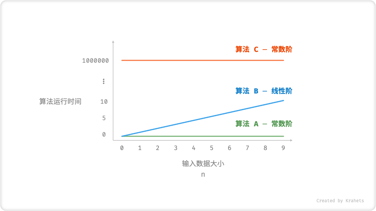
Fig. 算法 A, B, C 的时间增长趋势

相比直接统计算法运行时间，时间复杂度分析的做法有什么好处呢？以及有什么不足？

时间复杂度可以有效评估算法效率。 算法 B 运行时间的增长是线性的，在 $n > 1$ 时慢于算法 A ，在 $n > 1000000$ 时慢于算法 C 。实质上，只要输入数据大小 $n$ 足够大，复杂度为「常数阶」的算法一定优于「线性阶」的算法，这也正是时间增长趋势的含义。

时间复杂度分析将统计「计算操作的运行时间」简化为统计「计算操作的数量」。 这是因为，无论是运行平台、还是计算操作类型，都与算法运行时间的增长趋势无关。因此，我们可以简单地将所有计算操作的执行时间统一看作是相同的 “单位时间” 。

时间复杂度也存在一定的局限性。 比如，虽然算法 A 和 C 的时间复杂度相同，但是实际的运行时间有非常大的差别。再比如，虽然算法 B 比 C 的时间复杂度要更高，但在输入数据大小 $n$ 比较小时，算法 B 是要明显优于算法 C 的。即使存在这些问题，计算复杂度仍然是评判算法效率的最有效、最常用方法。

函数渐近上界¶

设算法「计算操作数量」为 $T(n)$ ，其是一个关于输入数据大小 $n$ 的函数。例如，以下算法的操作数量为

\[ T(n) = 3 + 2n \]

JavaC++PythonGoJavaScriptTypeScriptCC#

void algorithm(int n) {
    int a = 1;  // +1
    a = a + 1;  // +1
    a = a * 2;  // +1
    // 循环 n 次
    for (int i = 0; i < n; i++) { // +1（每轮都执行 i ++）
        System.out.println(0);    // +1
    }
}

void algorithm(int n) {
    int a = 1;  // +1
    a = a + 1;  // +1
    a = a * 2;  // +1
    // 循环 n 次
    for (int i = 0; i < n; i++) { // +1（每轮都执行 i ++）
        cout << 0 << endl;    // +1
    }
}

def algorithm(n):
    a = 1  # +1
    a = a + 1  # +1
    a = a * 2  # +1
    # 循环 n 次
    for i in range(n):  # +1
        print(0)        # +1

func algorithm(n int) {
    a := 1      // +1
    a = a + 1   // +1
    a = a * 2   // +1
    // 循环 n 次
    for i := 0; i < n; i++ {    // +1
        fmt.Println(a)          // +1
    }   
}

$T(n)$ 是个一次函数，说明时间增长趋势是线性的，因此易得时间复杂度是线性阶。

我们将线性阶的时间复杂度记为 $O(n)$ ，这个数学符号被称为「大 $O$ 记号 Big-$O$ Notation」，代表函数 $T(n)$ 的「渐近上界 asymptotic upper bound」。

我们要推算时间复杂度，本质上是在计算「操作数量函数 $T(n)$ 」的渐近上界。下面我们先来看看函数渐近上界的数学定义。

函数渐近上界

若存在正实数 $c$ 和实数 $n_0$ ，使得对于所有的 $n > n_0$ ，均有 $$ T(n) \leq c \cdot f(n) $$ 则可认为 $f(n)$ 给出了 $T(n)$ 的一个渐近上界，记为 $$ T(n) = O(f(n)) $$

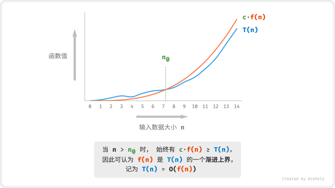
asymptotic_upper_bound

Fig. 函数的渐近上界

本质上看，计算渐近上界就是在找一个函数 $f(n)$ ，使得在 $n$ 趋向于无穷大时，$T(n)$ 和 $f(n)$ 处于相同的增长级别（仅相差一个常数项 $c$ 的倍数）。

Tip

渐近上界的数学味儿有点重，如果你感觉没有完全理解，无需担心，因为在实际使用中我们只需要会推算即可，数学意义可以慢慢领悟。

推算方法¶

推算出 $f(n)$ 后，我们就得到时间复杂度 $O(f(n))$ 。那么，如何来确定渐近上界 $f(n)$ 呢？总体分为两步，首先「统计操作数量」，然后「判断渐近上界」。

1. 统计操作数量¶

对着代码，从上到下一行一行地计数即可。然而，由于上述 $c \cdot f(n)$ 中的常数项 $c$ 可以取任意大小，因此操作数量 $T(n)$ 中的各种系数、常数项都可以被忽略。根据此原则，可以总结出以下计数偷懒技巧：

跳过数量与 $n$ 无关的操作。 因为他们都是 $T(n)$ 中的常数项，对时间复杂度不产生影响。
省略所有系数。 例如，循环 $2n$ 次、$5n + 1$ 次、……，都可以化简记为 $n$ 次，因为 $n$ 前面的系数对时间复杂度也不产生影响。
循环嵌套时使用乘法。 总操作数量等于外层循环和内层循环操作数量之积，每一层循环依然可以分别套用上述 1. 和 2. 技巧。

根据以下示例，使用上述技巧前、后的统计结果分别为

\[ \begin{aligned} T(n) & = 2n(n + 1) + (5n + 1) + 2 & \text{完整统计 (-.-|||)} \newline & = 2n^2 + 7n + 3 \newline T(n) & = n^2 + n & \text{偷懒统计 (o.O)} \end{aligned} \]

最终，两者都能推出相同的时间复杂度结果，即 $O(n^2)$ 。

JavaC++PythonGoJavaScriptTypeScriptCC#

void algorithm(int n) {
    int a = 1;  // +0（技巧 1）
    a = a + n;  // +0（技巧 1）
    // +n（技巧 2）
    for (int i = 0; i < 5 * n + 1; i++) {
        System.out.println(0);
    }
    // +n*n（技巧 3）
    for (int i = 0; i < 2 * n; i++) {
        for (int j = 0; j < n + 1; j++) {
            System.out.println(0);
        }
    }
}

void algorithm(int n) {
    int a = 1;  // +0（技巧 1）
    a = a + n;  // +0（技巧 1）
    // +n（技巧 2）
    for (int i = 0; i < 5 * n + 1; i++) {
        cout << 0 << endl;
    }
    // +n*n（技巧 3）
    for (int i = 0; i < 2 * n; i++) {
        for (int j = 0; j < n + 1; j++) {
            cout << 0 << endl;
        }
    }
}

def algorithm(n):
    a = 1      # +0（技巧 1）
    a = a + n  # +0（技巧 1）
    # +n（技巧 2）
    for i in range(5 * n + 1):
        print(0)
    # +n*n（技巧 3）
    for i in range(2 * n):
        for j in range(n + 1):
            print(0)

func algorithm(n int) {
    a := 1      // +0（技巧 1）
    a = a + n  // +0（技巧 1）
    // +n（技巧 2）
    for i := 0; i < 5 * n + 1; i++ {
        fmt.Println(0)
    }
    // +n*n（技巧 3）
    for i := 0; i < 2 * n; i++ {
        for j := 0; j < n + 1; j++ {
            fmt.Println(0)
        }
    }
}

2. 判断渐近上界¶

时间复杂度由多项式 $T(n)$ 中最高阶的项来决定。这是因为在 $n$ 趋于无穷大时，最高阶的项将处于主导作用，其它项的影响都可以被忽略。

以下表格给出了一些例子，其中有一些夸张的值，是想要向大家强调 系数无法撼动阶数 这一结论。在 $n$ 趋于无穷大时，这些常数都是 “浮云” 。

操作数量 $T(n)$	时间复杂度 $O(f(n))$
$100000$	$O(1)$
$3n + 2$	$O(n)$
$2n^2 + 3n + 2$	$O(n^2)$
$n^3 + 10000n^2$	$O(n^3)$
$2^n + 10000n^{10000}$	$O(2^n)$

常见类型¶

设输入数据大小为 $n$ ，常见的时间复杂度类型有（从低到高排列）

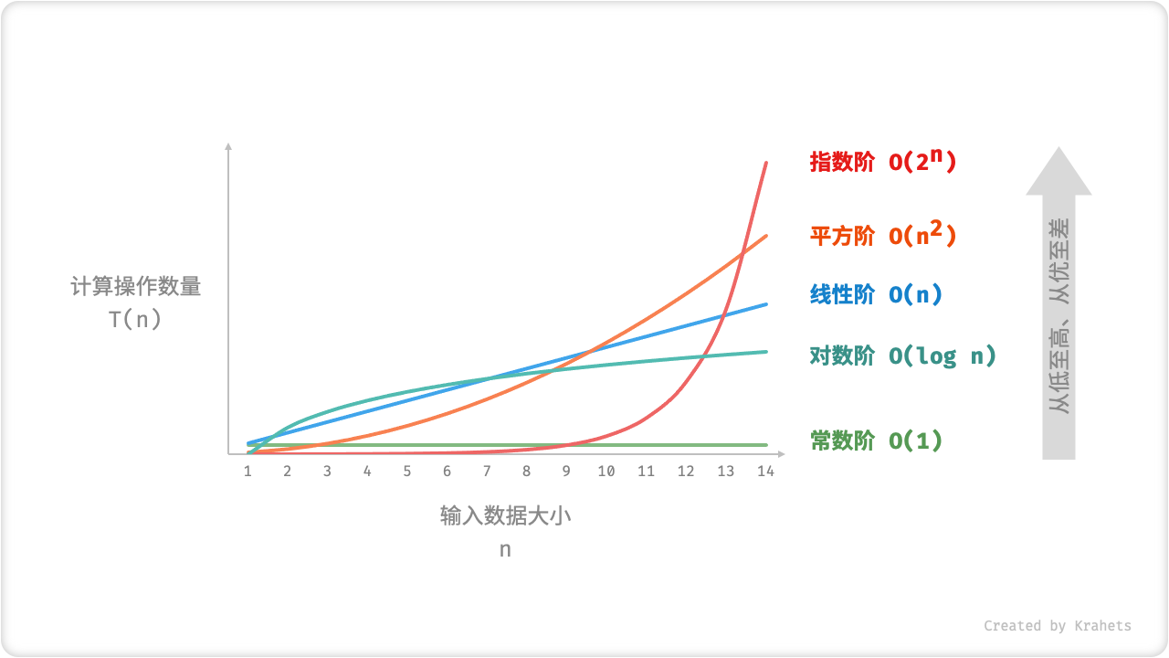
\[ \begin{aligned} O(1) < O(\log n) < O(n) < O(n \log n) < O(n^2) < O(2^n) < O(n!) \newline \text{常数阶} < \text{对数阶} < \text{线性阶} < \text{线性对数阶} < \text{平方阶} < \text{指数阶} < \text{阶乘阶} \end{aligned} \]

time_complexity_common_types

Fig. 时间复杂度的常见类型

Tip

部分示例代码需要一些前置知识，包括数组、递归算法等。如果遇到看不懂的地方无需担心，可以在学习完后面章节后再来复习，现阶段先聚焦在理解时间复杂度含义和推算方法上。

常数阶 $O(1)$¶

常数阶的操作数量与输入数据大小 $n$ 无关，即不随着 $n$ 的变化而变化。

对于以下算法，无论操作数量 size 有多大，只要与数据大小 $n$ 无关，时间复杂度就仍为 $O(1)$ 。

JavaC++PythonGoJavaScriptTypeScriptCC#

time_complexity.java

/* 常数阶 */
int constant(int n) {
    int count = 0;
    int size = 100000;
    for (int i = 0; i < size; i++)
        count++;
    return count;
}

time_complexity.cpp

/* 常数阶 */
int constant(int n) {
    int count = 0;
    int size = 100000;
    for (int i = 0; i < size; i++)
        count++;
    return count;
}

time_complexity.py

""" 常数阶 """
def constant(n):
    count = 0
    size = 100000
    for _ in range(size):
        count += 1
    return count

time_complexity.go

/* 常数阶 */
func constant(n int) int {
    count := 0
    size := 100000
    for i := 0; i < size; i++ {
        count ++
    }
    return count
}

time_complexity.js

time_complexity.ts

time_complexity.c

time_complexity.cs

线性阶 $O(n)$¶

线性阶的操作数量相对输入数据大小成线性级别增长。线性阶常出现于单层循环。

JavaC++PythonGoJavaScriptTypeScriptCC#

time_complexity.java

/* 线性阶 */
int linear(int n) {
    int count = 0;
    for (int i = 0; i < n; i++)
        count++;
    return count;
}

time_complexity.cpp

/* 线性阶 */
int linear(int n) {
    int count = 0;
    for (int i = 0; i < n; i++)
        count++;
    return count;
}

time_complexity.py

""" 线性阶 """
def linear(n):
    count = 0
    for _ in range(n):
        count += 1
    return count

time_complexity.go

/* 线性阶 */
func linear(n int) int {
    count := 0
    for i := 0; i < n; i++ {
        count++
    }
    return count
}

time_complexity.js

time_complexity.ts

time_complexity.c

time_complexity.cs

「遍历数组」和「遍历链表」等操作，时间复杂度都为 $O(n)$ ，其中 $n$ 为数组或链表的长度。

Tip

数据大小 $n$ 是根据输入数据的类型来确定的。 比如，在上述示例中，我们直接将 $n$ 看作输入数据大小；以下遍历数组示例中，数据大小 $n$ 为数组的长度。

JavaC++PythonGoJavaScriptTypeScriptCC#

time_complexity.java

/* 线性阶（遍历数组） */
int arrayTraversal(int[] nums) {
    int count = 0;
    // 循环次数与数组长度成正比
    for (int num : nums) {
        count++;
    }
    return count;
}

time_complexity.cpp

/* 线性阶（遍历数组） */
int arrayTraversal(vector<int>& nums) {
    int count = 0;
    // 循环次数与数组长度成正比
    for (int num : nums) {
        count++;
    }
    return count;
}

time_complexity.py

""" 线性阶（遍历数组）"""
def array_traversal(nums):
    count = 0
    # 循环次数与数组长度成正比
    for num in nums:
        count += 1
    return count

time_complexity.go

/* 线性阶（遍历数组） */
func arrayTraversal(nums []int) int {
    count := 0
    // 循环次数与数组长度成正比
    for range nums {
        count++
    }
    return count
}

time_complexity.js

time_complexity.ts

time_complexity.c

time_complexity.cs

平方阶 $O(n^2)$¶

平方阶的操作数量相对输入数据大小成平方级别增长。平方阶常出现于嵌套循环，外层循环和内层循环都为 $O(n)$ ，总体为 $O(n^2)$ 。

JavaC++PythonGoJavaScriptTypeScriptCC#

time_complexity.java

/* 平方阶 */
int quadratic(int n) {
    int count = 0;
    // 循环次数与数组长度成平方关系
    for (int i = 0; i < n; i++) {
        for (int j = 0; j < n; j++) {
            count++;
        }
    }
    return count;
}

time_complexity.cpp

/* 平方阶 */
int quadratic(int n) {
    int count = 0;
    // 循环次数与数组长度成平方关系
    for (int i = 0; i < n; i++) {
        for (int j = 0; j < n; j++) {
            count++;
        }
    }
    return count;
}

time_complexity.py

""" 平方阶 """
def quadratic(n):
    count = 0
    # 循环次数与数组长度成平方关系
    for i in range(n):
        for j in range(n):
            count += 1
    return count

time_complexity.go

/* 平方阶 */
func quadratic(n int) int {
    count := 0
    // 循环次数与数组长度成平方关系
    for i := 0; i < n; i++ {
        for j := 0; j < n; j++ {
            count++
        }
    }
    return count
}

time_complexity.js

time_complexity.ts

time_complexity.c

time_complexity.cs

time_complexity_constant_linear_quadratic

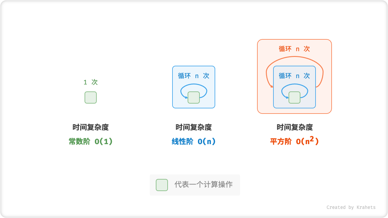
Fig. 常数阶、线性阶、平方阶的时间复杂度

以「冒泡排序」为例，外层循环 $n - 1$ 次，内层循环 $n-1, n-2, \cdots, 2, 1$ 次，平均为 $\frac{n}{2}$ 次，因此时间复杂度为 $O(n^2)$ 。

\[ O((n - 1) \frac{n}{2}) = O(n^2) \]

JavaC++PythonGoJavaScriptTypeScriptCC#

time_complexity.java

/* 平方阶（冒泡排序） */
int bubbleSort(int[] nums) {
    int count = 0;  // 计数器
    // 外循环：待排序元素数量为 n-1, n-2, ..., 1
    for (int i = nums.length - 1; i > 0; i--) {
        // 内循环：冒泡操作
        for (int j = 0; j < i; j++) {
            if (nums[j] > nums[j + 1]) {
                // 交换 nums[j] 与 nums[j + 1]
                int tmp = nums[j];
                nums[j] = nums[j + 1];
                nums[j + 1] = tmp;
                count += 3;  // 元素交换包含 3 个单元操作
            }
        }
    }
    return count;
}

time_complexity.cpp

/* 平方阶（冒泡排序） */
int bubbleSort(vector<int>& nums) {
    int count = 0;  // 计数器
    // 外循环：待排序元素数量为 n-1, n-2, ..., 1
    for (int i = nums.size() - 1; i > 0; i--) {
        // 内循环：冒泡操作
        for (int j = 0; j < i; j++) {
            if (nums[j] > nums[j + 1]) {
                // 交换 nums[j] 与 nums[j + 1]
                int tmp = nums[j];
                nums[j] = nums[j + 1];
                nums[j + 1] = tmp;
                count += 3;  // 元素交换包含 3 个单元操作
            }
        }
    }
    return count;
}

time_complexity.py

""" 平方阶（冒泡排序）"""
def bubble_sort(nums):
    count = 0  # 计数器
    # 外循环：待排序元素数量为 n-1, n-2, ..., 1
    for i in range(len(nums) - 1, 0, -1):
        # 内循环：冒泡操作
        for j in range(i):
            if nums[j] > nums[j + 1]:
                # 交换 nums[j] 与 nums[j + 1]
                tmp = nums[j]
                nums[j] = nums[j + 1]
                nums[j + 1] = tmp
                count += 3  # 元素交换包含 3 个单元操作
    return count

time_complexity.go

 /* 平方阶（冒泡排序） */
 func bubbleSort(nums []int) int {
    count := 0 // 计数器
    // 外循环：待排序元素数量为 n-1, n-2, ..., 1
    for i := len(nums) - 1; i > 0; i-- {
        // 内循环：冒泡操作
        for j := 0; j < i; j++ {
            if nums[j] > nums[j+1] {
                // 交换 nums[j] 与 nums[j + 1]
                tmp := nums[j]
                nums[j] = nums[j+1]
                nums[j+1] = tmp
                count += 3 // 元素交换包含 3 个单元操作
            }
        }
    }
    return count
}

time_complexity.js

time_complexity.ts

time_complexity.c

time_complexity.cs

指数阶 $O(2^n)$¶

Note

生物学科中的 “细胞分裂” 即是指数阶增长：初始状态为 $1$ 个细胞，分裂一轮后为 $2$ 个，分裂两轮后为 $4$ 个，……，分裂 $n$ 轮后有 $2^n$ 个细胞。

指数阶增长得非常快，在实际应用中一般是不能被接受的。若一个问题使用「暴力枚举」求解的时间复杂度是 $O(2^n)$ ，那么一般都需要使用「动态规划」或「贪心算法」等算法来求解。

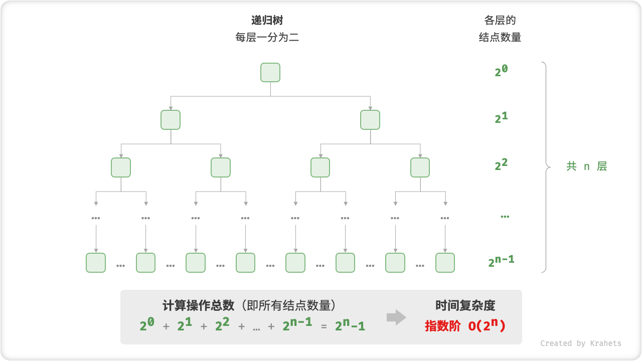
JavaC++PythonGoJavaScriptTypeScriptCC#

time_complexity.java

/* 指数阶（循环实现） */
int exponential(int n) {
    int count = 0, base = 1;
    // cell 每轮一分为二，形成数列 1, 2, 4, 8, ..., 2^(n-1)
    for (int i = 0; i < n; i++) {
        for (int j = 0; j < base; j++) {
            count++;
        }
        base *= 2;
    }
    // count = 1 + 2 + 4 + 8 + .. + 2^(n-1) = 2^n - 1
    return count;
}

time_complexity.cpp

/* 指数阶（循环实现） */
int exponential(int n) {
    int count = 0, base = 1;
    // cell 每轮一分为二，形成数列 1, 2, 4, 8, ..., 2^(n-1)
    for (int i = 0; i < n; i++) {
        for (int j = 0; j < base; j++) {
            count++;
        }
        base *= 2;
    }
    // count = 1 + 2 + 4 + 8 + .. + 2^(n-1) = 2^n - 1
    return count;
}

time_complexity.py

""" 指数阶（循环实现）"""
def exponential(n):
    count, base = 0, 1
    # cell 每轮一分为二，形成数列 1, 2, 4, 8, ..., 2^(n-1)
    for _ in range(n):
        for _ in range(base):
            count += 1
        base *= 2
    # count = 1 + 2 + 4 + 8 + .. + 2^(n-1) = 2^n - 1
    return count

time_complexity.go

/* 指数阶（循环实现）*/
func exponential(n int) int {
    count, base := 0, 1
    // cell 每轮一分为二，形成数列 1, 2, 4, 8, ..., 2^(n-1)
    for i := 0; i < n; i++ {
        for j := 0; j < base; j++ {
            count++
        }
        base *= 2
    }
    // count = 1 + 2 + 4 + 8 + .. + 2^(n-1) = 2^n - 1
    return count
}

time_complexity.js

time_complexity.ts

time_complexity.c

time_complexity.cs

time_complexity_exponential

Fig. 指数阶的时间复杂度

在实际算法中，指数阶常出现于递归函数。例如以下代码，不断地一分为二，分裂 $n$ 次后停止。

JavaC++PythonGoJavaScriptTypeScriptCC#

time_complexity.java

/* 指数阶（递归实现） */
int expRecur(int n) {
    if (n == 1) return 1;
    return expRecur(n - 1) + expRecur(n - 1) + 1;
}

time_complexity.cpp

/* 指数阶（递归实现） */
int expRecur(int n) {
    if (n == 1) return 1;
    return expRecur(n - 1) + expRecur(n - 1) + 1;
}

time_complexity.py

""" 指数阶（递归实现）"""
def exp_recur(n):
    if n == 1: return 1
    return exp_recur(n - 1) + exp_recur(n - 1) + 1

time_complexity.go

/* 指数阶（递归实现）*/
func expRecur(n int) int {
    if n == 1 {
        return 1
    }
    return expRecur(n-1) + expRecur(n-1) + 1
}

time_complexity.js

time_complexity.ts

time_complexity.c

time_complexity.cs

对数阶 $O(\log n)$¶

对数阶与指数阶正好相反，后者反映 “每轮增加到两倍的情况” ，而前者反映 “每轮缩减到一半的情况” 。对数阶仅次于常数阶，时间增长的很慢，是理想的时间复杂度。

对数阶常出现于「二分查找」和「分治算法」中，体现 “一分为多” 、“化繁为简” 的算法思想。

设输入数据大小为 $n$ ，由于每轮缩减到一半，因此循环次数是 $\log_2 n$ ，即 $2^n$ 的反函数。

JavaC++PythonGoJavaScriptTypeScriptCC#

time_complexity.java

/* 对数阶（循环实现） */
int logarithmic(float n) {
    int count = 0;
    while (n > 1) {
        n = n / 2;
        count++;
    }
    return count;
}

time_complexity.cpp

/* 对数阶（循环实现） */
int logarithmic(float n) {
    int count = 0;
    while (n > 1) {
        n = n / 2;
        count++;
    }
    return count;
}

time_complexity.py

""" 对数阶（循环实现）"""
def logarithmic(n):
    count = 0
    while n > 1:
        n = n / 2
        count += 1
    return count

time_complexity.go

/* 对数阶（循环实现）*/
func logarithmic(n float64) int {
    count := 0
    for n > 1 {
        n = n / 2
        count++
    }
    return count
}

time_complexity.js

time_complexity.ts

time_complexity.c

time_complexity.cs

time_complexity_logarithmic

Fig. 对数阶的时间复杂度

与指数阶类似，对数阶也常出现于递归函数。以下代码形成了一个高度为 $\log_2 n$ 的递归树。

JavaC++PythonGoJavaScriptTypeScriptCC#

time_complexity.java

/* 对数阶（递归实现） */
int logRecur(float n) {
    if (n <= 1) return 0;
    return logRecur(n / 2) + 1;
}

time_complexity.cpp

/* 对数阶（递归实现） */
int logRecur(float n) {
    if (n <= 1) return 0;
    return logRecur(n / 2) + 1;
}

time_complexity.py

""" 对数阶（递归实现）"""
def log_recur(n):
    if n <= 1: return 0
    return log_recur(n / 2) + 1

time_complexity.go

/* 对数阶（递归实现）*/
func logRecur(n float64) int {
    if n <= 1 {
        return 0
    }
    return logRecur(n/2) + 1
}

time_complexity.js

time_complexity.ts

time_complexity.c

time_complexity.cs

线性对数阶 $O(n \log n)$¶

线性对数阶常出现于嵌套循环中，两层循环的时间复杂度分别为 $O(\log n)$ 和 $O(n)$ 。

主流排序算法的时间复杂度都是 $O(n \log n )$ ，例如快速排序、归并排序、堆排序等。

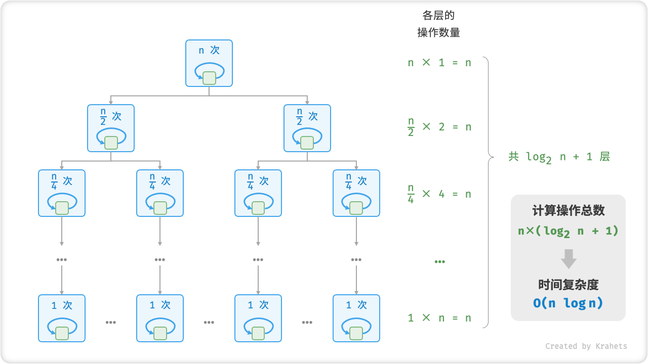
JavaC++PythonGoJavaScriptTypeScriptCC#

time_complexity.java

/* 线性对数阶 */
int linearLogRecur(float n) {
    if (n <= 1) return 1;
    int count = linearLogRecur(n / 2) + 
                linearLogRecur(n / 2);
    for (int i = 0; i < n; i++) {
        count++;
    }
    return count;
}

time_complexity.cpp

/* 线性对数阶 */
int linearLogRecur(float n) {
    if (n <= 1) return 1;
    int count = linearLogRecur(n / 2) + 
                linearLogRecur(n / 2);
    for (int i = 0; i < n; i++) {
        count++;
    }
    return count;
}

time_complexity.py

""" 线性对数阶 """
def linear_log_recur(n):
    if n <= 1: return 1
    count = linear_log_recur(n // 2) + \
            linear_log_recur(n // 2)
    for _ in range(n):
        count += 1
    return count

time_complexity.go

/* 线性对数阶 */
func linearLogRecur(n float64) int {
    if n <= 1 {
        return 1
    }
    count := linearLogRecur(n/2) +
        linearLogRecur(n/2)
    for i := 0.0; i < n; i++ {
        count++
    }
    return count
}

time_complexity.js

time_complexity.ts

time_complexity.c

time_complexity.cs

time_complexity_logarithmic_linear

Fig. 线性对数阶的时间复杂度

阶乘阶 $O(n!)$¶

阶乘阶对应数学上的「全排列」。即给定 $n$ 个互不重复的元素，求其所有可能的排列方案，则方案数量为

\[ n! = n \times (n - 1) \times (n - 2) \times \cdots \times 2 \times 1 \]

阶乘常使用递归实现。例如以下代码，第一层分裂出 $n$ 个，第二层分裂出 $n - 1$ 个，…… ，直至到第 $n$ 层时终止分裂。

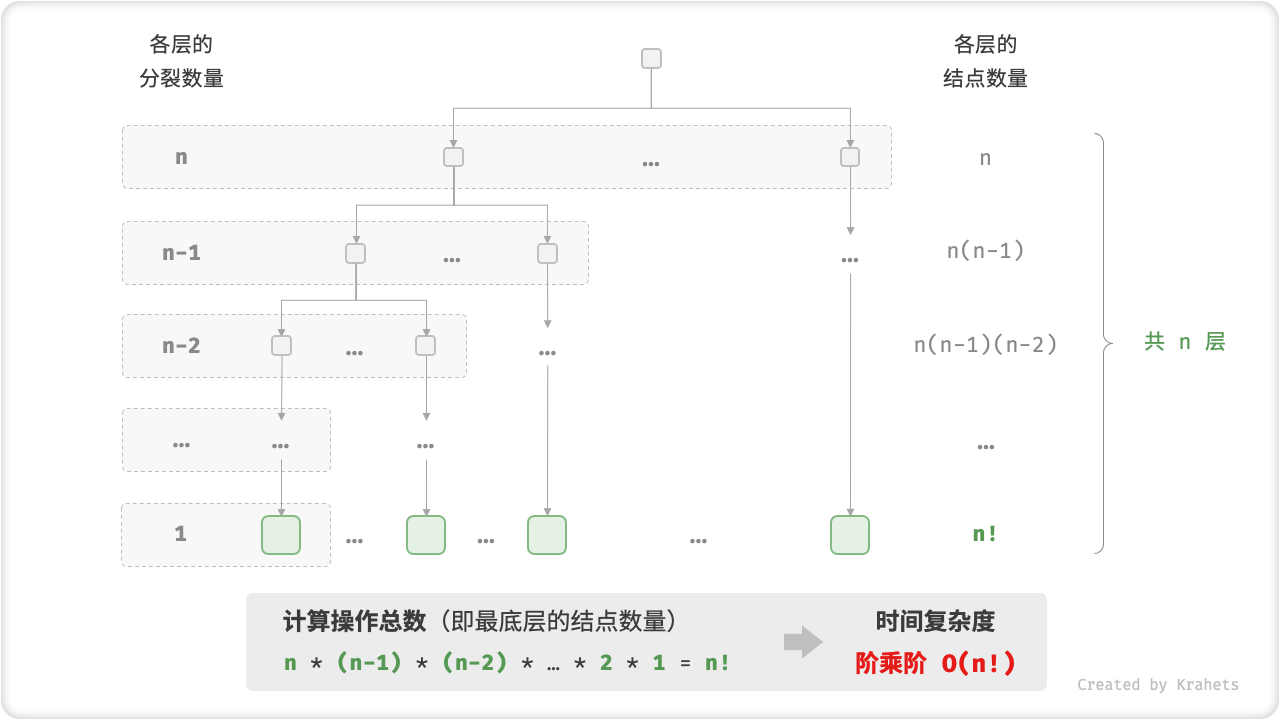
JavaC++PythonGoJavaScriptTypeScriptCC#

time_complexity.java

/* 阶乘阶（递归实现） */
int factorialRecur(int n) {
    if (n == 0) return 1;
    int count = 0;
    // 从 1 个分裂出 n 个
    for (int i = 0; i < n; i++) {
        count += factorialRecur(n - 1);
    }
    return count;
}

time_complexity.cpp

/* 阶乘阶（递归实现） */
int factorialRecur(int n) {
    if (n == 0) return 1;
    int count = 0;
    // 从 1 个分裂出 n 个
    for (int i = 0; i < n; i++) {
        count += factorialRecur(n - 1);
    }
    return count;
}

time_complexity.py

""" 阶乘阶（递归实现）"""
def factorial_recur(n):
    if n == 0: return 1
    count = 0
    # 从 1 个分裂出 n 个
    for _ in range(n):
        count += factorial_recur(n - 1)
    return count

time_complexity.go

/* 阶乘阶（递归实现） */
func factorialRecur(n int) int {
    if n == 0 {
        return 1
    }
    count := 0
    // 从 1 个分裂出 n 个
    for i := 0; i < n; i++ {
        count += factorialRecur(n - 1)
    }
    return count
}

time_complexity.js

time_complexity.ts

time_complexity.c

time_complexity.cs

time_complexity_factorial

Fig. 阶乘阶的时间复杂度

最差、最佳、平均时间复杂度¶

某些算法的时间复杂度不是恒定的，而是与输入数据的分布有关。 举一个例子，输入一个长度为 $n$ 数组 nums ，其中 nums 由从 $1$ 至 $n$ 的数字组成，但元素顺序是随机打乱的；算法的任务是返回元素 $1$ 的索引。我们可以得出以下结论：

当 nums = [?, ?, ..., 1]，即当末尾元素是 $1$ 时，则需完整遍历数组，此时达到 最差时间复杂度 $O(n)$ ；
当 nums = [1, ?, ?, ...] ，即当首个数字为 $1$ 时，无论数组多长都不需要继续遍历，此时达到 最佳时间复杂度 $\Omega(1)$ ；

「函数渐近上界」使用大 $O$ 记号表示，代表「最差时间复杂度」。与之对应，「函数渐近下界」用 $\Omega$ 记号（Omega Notation）来表示，代表「最佳时间复杂度」。

JavaC++PythonGoJavaScriptTypeScriptCC#

worst_best_time_complexity.java

public class worst_best_time_complexity {
    /* 生成一个数组，元素为 { 1, 2, ..., n }，顺序被打乱 */
    static int[] randomNumbers(int n) {
        Integer[] nums = new Integer[n];
        // 生成数组 nums = { 1, 2, 3, ..., n }
        for (int i = 0; i < n; i++) {
            nums[i] = i + 1;
        }
        // 随机打乱数组元素
        Collections.shuffle(Arrays.asList(nums));
        // Integer[] -> int[]
        int[] res = new int[n];
        for (int i = 0; i < n; i++) {
            res[i] = nums[i];
        }
        return res;
    }

    /* 查找数组 nums 中数字 1 所在索引 */
    static int findOne(int[] nums) {
        for (int i = 0; i < nums.length; i++) {
            if (nums[i] == 1)
                return i;
        }
        return -1;
    }

    /* Driver Code */
    public static void main(String[] args) {
        for (int i = 0; i < 10; i++) {
            int n = 100;
            int[] nums = randomNumbers(n);
            int index = findOne(nums);
            System.out.println("打乱后的数组为 " + Arrays.toString(nums));
            System.out.println("数字 1 的索引为 " + index);
        }
    }
}

worst_best_time_complexity.cpp

/* 生成一个数组，元素为 { 1, 2, ..., n }，顺序被打乱 */
vector<int> randomNumbers(int n) {
    vector<int> nums(n);
    // 生成数组 nums = { 1, 2, 3, ..., n }
    for (int i = 0; i < n; i++) {
        nums[i] = i + 1;
    }
    // 使用系统时间生成随机种子
    unsigned seed = chrono::system_clock::now().time_since_epoch().count();
    // 随机打乱数组元素
    shuffle(nums.begin(), nums.end(), default_random_engine(seed));
    return nums;
}

/* 查找数组 nums 中数字 1 所在索引 */
int findOne(vector<int>& nums) {
    for (int i = 0; i < nums.size(); i++) {
        if (nums[i] == 1)
            return i;
    }
    return -1;
}


/* Driver Code */
int main() {
    for (int i = 0; i < 1000; i++) {
        int n = 100;
        vector<int> nums = randomNumbers(n);
        int index = findOne(nums);
        cout << "\n数组 [ 1, 2, ..., n ] 被打乱后 = ";
        PrintUtil::printVector(nums);
        cout << "数字 1 的索引为 " << index << endl;
    }
    return 0;
}

worst_best_time_complexity.py

""" 生成一个数组，元素为: 1, 2, ..., n ，顺序被打乱 """
def random_numbers(n):
    # 生成数组 nums =: 1, 2, 3, ..., n 
    nums = [i for i in range(1, n + 1)]
    # 随机打乱数组元素
    random.shuffle(nums)
    return nums

""" 查找数组 nums 中数字 1 所在索引 """
def find_one(nums):
    for i in range(len(nums)):
        if nums[i] == 1:
            return i
    return -1

""" Driver Code """
if __name__ == "__main__":
    for i in range(10):
        n = 100
        nums = random_numbers(n)
        index = find_one(nums)
        print("\n数组 [ 1, 2, ..., n ] 被打乱后 =", nums)
        print("数字 1 的索引为", index)

worst_best_time_complexity.go

/* 生成一个数组，元素为 { 1, 2, ..., n }，顺序被打乱 */
func randomNumbers(n int) []int {
    nums := make([]int, n)
    // 生成数组 nums = { 1, 2, 3, ..., n }
    for i := 0; i < n; i++ {
        nums[i] = i + 1
    }
    // 随机打乱数组元素
    rand.Shuffle(len(nums), func(i, j int) {
        nums[i], nums[j] = nums[j], nums[i]
    })
    return nums
}

/* 查找数组 nums 中数字 1 所在索引 */
func findOne(nums []int) int {
    for i := 0; i < len(nums); i++ {
        if nums[i] == 1 {
            return i
        }
    }
    return -1
}

/* Driver Code */
func main() {
    for i := 0; i < 10; i++ {
        n := 100
        nums := randomNumbers(n)
        index := findOne(nums)
        fmt.Println("\n数组 [ 1, 2, ..., n ] 被打乱后 =", nums)
        fmt.Println("数字 1 的索引为", index)
    }
}

worst_best_time_complexity.js

worst_best_time_complexity.ts

worst_best_time_complexity.c

worst_best_time_complexity.cs

Tip

我们在实际应用中很少使用「最佳时间复杂度」，因为往往只有很小概率下才能达到，会带来一定的误导性。反之，「最差时间复杂度」最为实用，因为它给出了一个 “效率安全值” ，让我们可以放心地使用算法。

从上述示例可以看出，最差或最佳时间复杂度只出现在 “特殊分布的数据” 中，这些情况的出现概率往往很小，因此并不能最真实地反映算法运行效率。相对地，「平均时间复杂度」可以体现算法在随机输入数据下的运行效率，用 $\Theta$ 记号（Theta Notation）来表示。

对于部分算法，我们可以简单地推算出随机数据分布下的平均情况。比如上述示例，由于输入数组是被打乱的，因此元素 $1$ 出现在任意索引的概率都是相等的，那么算法的平均循环次数则是数组长度的一半 $\frac{n}{2}$ ，平均时间复杂度为 $\Theta(\frac{n}{2}) = \Theta(n)$ 。

但在实际应用中，尤其是较为复杂的算法，计算平均时间复杂度比较困难，因为很难简便地分析出在数据分布下的整体数学期望。这种情况下，我们一般使用最差时间复杂度来作为算法效率的评判标准。

为什么很少看到 $\Theta$ 符号？

实际中我们经常使用「大 $O$ 符号」来表示「平均复杂度」，这样严格意义上来说是不规范的。这可能是因为 $O$ 符号实在是太朗朗上口了。
如果在本书和其他资料中看到类似 平均时间复杂度 $O(n)$ 的表述，请你直接理解为 $\Theta(n)$ 即可。

操作数量 \(T(n)\)	时间复杂度 \(O(f(n))\)
\(100000\)	\(O(1)\)
\(3n + 2\)	\(O(n)\)
\(2n^2 + 3n + 2\)	\(O(n^2)\)
\(n^3 + 10000n^2\)	\(O(n^3)\)
\(2^n + 10000n^{10000}\)	\(O(2^n)\)

时间复杂度¶

统计算法运行时间¶

统计时间增长趋势¶

函数渐近上界¶

推算方法¶

1. 统计操作数量¶

2. 判断渐近上界¶

常见类型¶

常数阶 \(O(1)\)¶

线性阶 \(O(n)\)¶

平方阶 \(O(n^2)\)¶

指数阶 \(O(2^n)\)¶

对数阶 \(O(\log n)\)¶

线性对数阶 \(O(n \log n)\)¶

阶乘阶 \(O(n!)\)¶

最差、最佳、平均时间复杂度¶